Tidymodels
Math 150 - Spring 2023
Agenda
- Workflow to help us think about model building
- Breaking up data for independent assessment
- Assessment metrics
Comparing Models
Data Modeling: The analysis in this culture starts with assuming a stochastic data model for the inside of the black box…The values of the parameters are estimated from the data and the model then used for information and/or prediction
Algorithmic Modeling: The analysis in this culture considers the inside of the box complex and unknown. The approach is to find a function f(x) — an algorithm that operates on x to predict the responses y.
Reference: Leo Breiman (2001)
Data & goal
Data: Project FeederWatch#TidyTuesday dataset on Project FeederWatch, a citizen science project for bird science, by way of TidyTuesday.
Can the characteristics of the bird feeder site like the surrounding yard and habitat predict whether a bird feeder site will be used by squirrels?
Rows: 235,685
Columns: 59
$ squirrels                    <fct> no squirrels, no squirrels, no squirrels,…
$ yard_type_pavement           <dbl> 0, 0, 0, 0, 0, 0, 0, 0, 0, 0, 0, 0, 0, 0,…
$ yard_type_garden             <dbl> 0, 0, 0, 0, 0, 0, 0, 0, 0, 0, 0, 0, 0, 0,…
$ yard_type_landsca            <dbl> 1, 1, 1, 1, 1, 1, 0, 0, 0, 0, 1, 1, 1, 1,…
$ yard_type_woods              <dbl> 0, 0, 0, 0, 0, 0, 1, 1, 1, 1, 1, 1, 1, 1,…
$ yard_type_desert             <dbl> 0, 0, 0, 0, 0, 0, 0, 0, 0, 0, 0, 0, 0, 0,…
$ hab_dcid_woods               <dbl> 1, 1, 1, 1, 1, 1, 1, 1, 1, 1, NA, NA, NA,…
$ hab_evgr_woods               <dbl> NA, NA, NA, NA, 0, 0, NA, NA, NA, NA, NA,…
$ hab_mixed_woods              <dbl> 1, 1, 1, 1, 1, 1, NA, NA, NA, NA, 1, 1, 1…
$ hab_orchard                  <dbl> NA, NA, NA, NA, 0, 0, NA, NA, NA, NA, NA,…
$ hab_park                     <dbl> NA, NA, NA, NA, 0, 0, NA, NA, NA, NA, 1, …
$ hab_water_fresh              <dbl> 1, 1, 1, 1, 1, 1, 1, 1, 1, 1, 1, 1, 1, 1,…
$ hab_water_salt               <dbl> NA, NA, NA, NA, 0, 0, NA, NA, NA, NA, 1, …
$ hab_residential              <dbl> 1, 1, 1, 1, 1, 1, NA, NA, NA, NA, 1, 1, 1…
$ hab_industrial               <dbl> NA, NA, NA, NA, 0, 0, NA, NA, NA, NA, 1, …
$ hab_agricultural             <dbl> 1, 1, 1, 1, 1, 1, NA, NA, NA, NA, 1, 1, 1…
$ hab_desert_scrub             <dbl> NA, NA, NA, NA, 0, 0, NA, NA, NA, NA, NA,…
$ hab_young_woods              <dbl> NA, NA, NA, NA, 0, 0, NA, NA, NA, NA, NA,…
$ hab_swamp                    <dbl> NA, NA, NA, NA, 0, 0, NA, NA, NA, NA, NA,…
$ hab_marsh                    <dbl> 1, 1, 1, 1, 1, 1, NA, NA, NA, NA, 1, 1, 1…
$ evgr_trees_atleast           <dbl> 11, 11, 11, 11, 11, 11, 0, 0, 0, 4, 1, 1,…
$ evgr_shrbs_atleast           <dbl> 4, 4, 4, 4, 1, 1, 1, 1, 1, 1, 4, 4, 4, 4,…
$ dcid_trees_atleast           <dbl> 11, 11, 11, 11, 1, 1, 11, 11, 11, 11, 4, …
$ dcid_shrbs_atleast           <dbl> 4, 4, 4, 4, 4, 4, 11, 11, 11, 11, 4, 4, 4…
$ fru_trees_atleast            <dbl> 4, 4, 4, 4, 1, 1, 1, 1, 1, 1, 1, 1, 1, 1,…
$ cacti_atleast                <dbl> 0, 0, 0, 0, 0, 0, 0, 0, 0, 0, 0, 0, 0, 0,…
$ brsh_piles_atleast           <dbl> 0, 0, 0, 0, 0, 0, 1, 1, 1, 1, 1, 1, 1, 1,…
$ water_srcs_atleast           <dbl> 1, 1, 1, 1, 1, 1, 0, 0, 0, 0, 0, 0, 0, 0,…
$ bird_baths_atleast           <dbl> 0, 0, 0, 0, 0, 0, 1, 1, 1, 1, 0, 0, 0, 1,…
$ nearby_feeders               <dbl> 0, 1, 1, 1, 0, 0, 1, 0, 1, 1, 1, 1, 1, 1,…
$ cats                         <dbl> 0, 1, 1, 1, 1, 1, 1, 0, 0, 0, 1, 1, 1, 1,…
$ dogs                         <dbl> 0, 0, 0, 0, 0, 0, 1, 0, 0, 0, 1, 1, 1, 1,…
$ humans                       <dbl> 0, 0, 0, 0, 0, 1, 1, 1, 0, 1, 1, 1, 1, 1,…
$ housing_density              <dbl> 2, 2, 2, 2, 2, 2, 1, 1, 1, 1, 2, 2, 2, 2,…
$ fed_in_jan                   <dbl> 1, 1, 1, 1, 1, 1, 1, 1, 1, 1, 1, NA, 1, N…
$ fed_in_feb                   <dbl> 1, 1, 1, 1, 1, 1, 1, 1, 1, 1, 1, NA, 1, N…
$ fed_in_mar                   <dbl> 1, 1, 1, 1, 1, 1, 1, 1, 1, 1, 1, NA, 1, N…
$ fed_in_apr                   <dbl> 1, 1, 1, 1, 1, 0, 1, 1, 1, 1, 1, NA, 0, N…
$ fed_in_may                   <dbl> 0, 0, 0, 0, 0, 0, 1, 1, 1, 1, 0, NA, 0, N…
$ fed_in_jun                   <dbl> 0, 0, 0, 0, 0, 0, 1, 1, 1, 1, 0, NA, 0, N…
$ fed_in_jul                   <dbl> 0, 0, 0, 0, 0, 0, 1, 1, 1, 1, 0, NA, 0, N…
$ fed_in_aug                   <dbl> 0, 0, 0, 0, 0, 0, 1, 1, 1, 1, 0, NA, 0, N…
$ fed_in_sep                   <dbl> 0, 0, 0, 0, 0, 0, 1, 1, 1, 1, 0, NA, 0, N…
$ fed_in_oct                   <dbl> 0, 0, 0, 0, 0, 0, 1, 1, 1, 1, 0, NA, 1, N…
$ fed_in_nov                   <dbl> 1, 1, 1, 1, 1, 1, 1, 1, 1, 1, 1, NA, 1, N…
$ fed_in_dec                   <dbl> 1, 1, 1, 1, 1, 1, 1, 1, 1, 1, 1, NA, 1, N…
$ numfeeders_suet              <dbl> 1, 1, 1, 1, 1, 1, 3, 3, 3, 3, 1, 1, 1, 2,…
$ numfeeders_ground            <dbl> NA, 0, 0, 0, NA, NA, 1, 1, 1, 1, 3, 3, 3,…
$ numfeeders_hanging           <dbl> 1, 1, 1, 3, NA, NA, 2, 2, 2, 2, 2, 2, 1, …
$ numfeeders_platfrm           <dbl> 1, 1, 1, 0, NA, NA, 1, 1, 1, 2, 1, 1, 1, …
$ numfeeders_humming           <dbl> NA, 0, 0, 0, NA, NA, 1, 1, 1, 1, NA, 0, 0…
$ numfeeders_water             <dbl> 1, 1, 1, 1, NA, NA, 2, 2, 2, 2, 1, 1, 1, …
$ numfeeders_thistle           <dbl> NA, 0, 0, 0, NA, NA, 1, 1, 1, 2, 1, 1, 1,…
$ numfeeders_fruit             <dbl> NA, 0, 0, 0, NA, NA, 1, 1, 1, 1, NA, 0, 0…
$ numfeeders_hopper            <dbl> NA, NA, NA, NA, 1, 1, NA, NA, NA, NA, NA,…
$ numfeeders_tube              <dbl> NA, NA, NA, NA, 1, 1, NA, NA, NA, NA, NA,…
$ numfeeders_other             <dbl> NA, NA, NA, NA, NA, NA, NA, NA, NA, NA, N…
$ population_atleast           <dbl> 1, 1, 1, 1, 1, 1, 1, 1, 1, 1, 5001, 5001,…
$ count_area_size_sq_m_atleast <dbl> 1.01, 1.01, 1.01, 1.01, 1.01, 1.01, 375.0…
Feeders
How are other characteristics related to the presence of squirrels?
# A tibble: 2 × 2
  squirrels    nearby_feeders
  <fct>                 <dbl>
1 no squirrels          0.344
2 squirrels             0.456
Other variables
What about some of the variables describing the habitat?
Modeling
Train / test
Create an initial split:
set.seed(470)
feeder_split <- site_data %>%
  initial_split(strata = squirrels) # prop = 3/4 in each group, by default
Save training data
feeder_train <- training(feeder_split)
dim(feeder_train)
[1] 176763 59Save testing data
feeder_test  <- testing(feeder_split)
dim(feeder_test)
[1] 58922 59Training data
feeder_train# A tibble: 176,763 × 59
squirrels yard_t…¹ yard_…² yard_…³ yard_…⁴ yard_…⁵ hab_d…⁶ hab_e…⁷ hab_m…⁸
<fct> <dbl> <dbl> <dbl> <dbl> <dbl> <dbl> <dbl> <dbl>
1 no squirrels 0 0 1 0 0 1 NA 1
2 no squirrels 0 0 1 0 0 1 NA 1
3 no squirrels 0 0 1 0 0 1 0 1
4 no squirrels 0 0 1 0 0 1 NA NA
5 no squirrels 0 0 1 1 0 1 0 0
6 no squirrels 0 0 1 0 0 1 NA 1
7 no squirrels 0 0 0 1 0 0 0 1
8 no squirrels 0 0 1 1 0 NA NA NA
9 no squirrels 0 0 1 0 0 1 1 NA
10 no squirrels 0 0 1 1 0 0 0 1
# … with 176,753 more rows, 50 more variables: hab_orchard <dbl>,
# hab_park <dbl>, hab_water_fresh <dbl>, hab_water_salt <dbl>,
# hab_residential <dbl>, hab_industrial <dbl>, hab_agricultural <dbl>,
# hab_desert_scrub <dbl>, hab_young_woods <dbl>, hab_swamp <dbl>,
# hab_marsh <dbl>, evgr_trees_atleast <dbl>, evgr_shrbs_atleast <dbl>,
# dcid_trees_atleast <dbl>, dcid_shrbs_atleast <dbl>,
# fru_trees_atleast <dbl>, cacti_atleast <dbl>, brsh_piles_atleast <dbl>, …Feature engineering
We prefer simple models when possible, but parsimony does not mean sacrificing accuracy (or predictive performance) in the interest of simplicity
Variables that go into the model and how they are represented are just as critical to success of the model
Feature engineering allows us to get creative with our predictors in an effort to make them more useful for our model (to increase its predictive performance)
Modeling workflow
Create a recipe for feature engineering steps to be applied to the training data
Fit the model to the training data after these steps have been applied
Using the model estimates from the training data, predict outcomes for the test data
Evaluate the performance of the model on the test data
Building recipes
Initiate a recipe
Working with recipes
- When building recipes you in a pipeline, you don’t get to see the effect of the recipe on your data, which can be unsettling
- You can take a peek at what will happen when you ultimately apply the recipe to your data at the time of fitting the model
- This requires two functions:
prep()to train the recipe andbake()to apply it to your data
. . .
Note
Using prep() and bake() are shown here for demonstrative purposes. They do not need to be a part of your pipeline. I do find them assuring, however, so that I can see the effects of the recipe steps as the recipe is built.
Impute missing values & Remove zero variance predictors
Impute missing values (replace with mean).
Remove all predictors that contain only a single value
Prep and bake
feeder_rec_trained <- prep(feeder_rec)

bake(feeder_rec_trained, feeder_train) %>%
  glimpse()
Rows: 176,763
Columns: 59
$ yard_type_pavement <dbl> 0, 0, 0, 0, 0, 0, 0, 0, 0, 0, 0, 0, 0, 0,…
$ yard_type_garden <dbl> 0, 0, 0, 0, 0, 0, 0, 0, 0, 0, 0, 0, 0, 0,…
$ yard_type_landsca <dbl> 1, 1, 1, 1, 1, 1, 0, 1, 1, 1, 1, 1, 1, 1,…
$ yard_type_woods <dbl> 0, 0, 0, 0, 1, 0, 1, 1, 0, 1, 0, 1, 1, 0,…
$ yard_type_desert <dbl> 0, 0, 0, 0, 0, 0, 0, 0, 0, 0, 0, 0, 0, 0,…
$ hab_dcid_woods <dbl> 1.0000000, 1.0000000, 1.0000000, 1.000000…
$ hab_evgr_woods <dbl> 0.223341, 0.223341, 0.000000, 0.223341, 0…
$ hab_mixed_woods <dbl> 1.000000, 1.000000, 1.000000, 0.655411, 0…
$ hab_orchard <dbl> 0.09324933, 0.09324933, 0.00000000, 0.093…
$ hab_park <dbl> 0.4502185, 0.4502185, 0.0000000, 0.450218…
$ hab_water_fresh <dbl> 1.0000000, 1.0000000, 1.0000000, 1.000000…
$ hab_water_salt <dbl> 0.05016023, 0.05016023, 0.00000000, 0.050…
$ hab_residential <dbl> 1.0000000, 1.0000000, 1.0000000, 1.000000…
$ hab_industrial <dbl> 0.2215792, 0.2215792, 0.0000000, 0.221579…
$ hab_agricultural <dbl> 1.0000000, 1.0000000, 1.0000000, 0.409835…
$ hab_desert_scrub <dbl> 0.09257371, 0.09257371, 0.00000000, 0.092…
$ hab_young_woods <dbl> 0.349782, 0.349782, 0.000000, 0.349782, 0…
$ hab_swamp <dbl> 0.2917369, 0.2917369, 0.0000000, 0.291736…
$ hab_marsh <dbl> 1.0000000, 1.0000000, 1.0000000, 0.175361…
$ evgr_trees_atleast <dbl> 11, 11, 11, 0, 11, 1, 4, 4, 4, 1, 1, 1, 1…
$ evgr_shrbs_atleast <dbl> 4, 4, 1, 4, 0, 1, 4, 4, 4, 1, 0, 4, 4, 11…
$ dcid_trees_atleast <dbl> 11, 11, 1, 4, 1, 4, 11, 11, 4, 1, 1, 1, 1…
$ dcid_shrbs_atleast <dbl> 4, 4, 4, 1, 1, 4, 11, 11, 1, 1, 0, 4, 4, …
$ fru_trees_atleast <dbl> 4.00000, 4.00000, 1.00000, 1.00000, 0.000…
$ cacti_atleast <dbl> 0.0000000, 0.0000000, 0.0000000, 0.000000…
$ brsh_piles_atleast <dbl> 0, 0, 0, 1, 0, 0, 1, 4, 1, 0, 0, 1, 1, 1,…
$ water_srcs_atleast <dbl> 1.0000000, 1.0000000, 1.0000000, 0.000000…
$ bird_baths_atleast <dbl> 0, 0, 0, 1, 0, 0, 1, 1, 4, 0, 0, 0, 0, 1,…
$ nearby_feeders <dbl> 1, 1, 0, 1, 0, 0, 0, 1, 1, 0, 0, 0, 0, 1,…
$ cats <dbl> 1, 1, 1, 1, 0, 0, 0, 1, 0, 1, 1, 0, 0, 0,…
$ dogs <dbl> 0, 0, 0, 1, 0, 0, 0, 1, 1, 1, 1, 1, 0, 1,…
$ humans <dbl> 0, 0, 1, 1, 1, 0, 0, 1, 1, 1, 1, 1, 1, 1,…
$ housing_density <dbl> 2, 2, 2, 2, 2, 3, 1, 1, 1, 1, 2, 1, 2, 2,…
$ fed_in_jan <dbl> 1.0000000, 1.0000000, 1.0000000, 1.000000…
$ fed_in_feb <dbl> 1.000000, 1.000000, 1.000000, 1.000000, 1…
$ fed_in_mar <dbl> 1.0000000, 1.0000000, 1.0000000, 1.000000…
$ fed_in_apr <dbl> 1.0000000, 1.0000000, 0.0000000, 1.000000…
$ fed_in_may <dbl> 0.0000000, 0.0000000, 0.0000000, 1.000000…
$ fed_in_jun <dbl> 0.0000000, 0.0000000, 0.0000000, 1.000000…
$ fed_in_jul <dbl> 0.000000, 0.000000, 0.000000, 1.000000, 1…
$ fed_in_aug <dbl> 0.0000000, 0.0000000, 0.0000000, 1.000000…
$ fed_in_sep <dbl> 0.0000000, 0.0000000, 0.0000000, 1.000000…
$ fed_in_oct <dbl> 0.0000000, 0.0000000, 0.0000000, 1.000000…
$ fed_in_nov <dbl> 1, 1, 1, 1, 1, 1, 1, 1, 1, 1, 1, 1, 1, 1,…
$ fed_in_dec <dbl> 1, 1, 1, 1, 1, 1, 1, 1, 1, 1, 1, 1, 1, 1,…
$ numfeeders_suet <dbl> 1, 1, 1, 2, 1, 1, 1, 1, 3, 2, 2, 3, 4, 1,…
$ numfeeders_ground <dbl> 0.000000, 0.000000, 1.270686, 1.000000, 0…
$ numfeeders_hanging <dbl> 1.000000, 1.000000, 2.707598, 2.000000, 2…
$ numfeeders_platfrm <dbl> 1.000000, 1.000000, 1.033629, 1.033629, 0…
$ numfeeders_humming <dbl> 0.0000000, 0.0000000, 0.4989854, 0.498985…
$ numfeeders_water <dbl> 1.0000000, 1.0000000, 0.7887147, 0.788714…
$ numfeeders_thistle <dbl> 0.000000, 0.000000, 1.007624, 1.000000, 1…
$ numfeeders_fruit <dbl> 0.0000000, 0.0000000, 0.1442454, 0.144245…
$ numfeeders_hopper <dbl> 1.385205, 1.385205, 1.000000, 1.385205, 0…
$ numfeeders_tube <dbl> 2.162308, 2.162308, 1.000000, 2.162308, 2…
$ numfeeders_other <dbl> 0.6037683, 0.6037683, 0.6037683, 0.603768…
$ population_atleast <dbl> 1, 1, 1, 25001, 5001, 25001, 1, 1, 1, 1, …
$ count_area_size_sq_m_atleast <dbl> 1.01, 1.01, 1.01, 1.01, 1.01, 1.01, 375.0…
$ squirrels <fct> no squirrels, no squirrels, no squirrels,…Building workflows
Specify model
feeder_log <- logistic_reg() %>%
  set_engine("glm")

feeder_log
Logistic Regression Model Specification (classification)
Computational engine: glm Build workflow
Workflows bring together models and recipes so that they can be easily applied to both the training and test data.
feeder_wflow <- workflow() %>%
add_recipe(feeder_rec) %>%
add_model(feeder_log) See next slide for workflow…
View workflow
feeder_wflow══ Workflow ════════════════════════════════════════════════════════════════════
Preprocessor: Recipe
Model: logistic_reg()
── Preprocessor ────────────────────────────────────────────────────────────────
2 Recipe Steps
• step_impute_mean()
• step_nzv()
── Model ───────────────────────────────────────────────────────────────────────
Logistic Regression Model Specification (classification)

Computational engine: glm Fit model to training data
feeder_fit <- feeder_wflow %>%
  fit(data = feeder_train)

feeder_fit %>% tidy()
# A tibble: 59 × 5
term estimate std.error statistic p.value
<chr> <dbl> <dbl> <dbl> <dbl>
1 (Intercept) -1.42 0.0505 -28.2 2.26e-174
2 yard_type_pavement -0.854 0.149 -5.74 9.23e- 9
3 yard_type_garden -0.175 0.0392 -4.47 7.89e- 6
4 yard_type_landsca 0.168 0.0219 7.69 1.45e- 14
5 yard_type_woods 0.309 0.0170 18.1 1.59e- 73
6 yard_type_desert -0.297 0.0789 -3.76 1.68e- 4
7 hab_dcid_woods 0.336 0.0161 20.9 6.55e- 97
8 hab_evgr_woods -0.0797 0.0192 -4.15 3.36e- 5
9 hab_mixed_woods 0.420 0.0158 26.5 3.17e-155
10 hab_orchard -0.307 0.0252 -12.2 4.00e- 34
# … with 49 more rows. . .
So many predictors!
Model fit summary
feeder_fit %>% tidy() # A tibble: 59 × 5
term estimate std.error statistic p.value
<chr> <dbl> <dbl> <dbl> <dbl>
1 (Intercept) -1.42 0.0505 -28.2 2.26e-174
2 yard_type_pavement -0.854 0.149 -5.74 9.23e- 9
3 yard_type_garden -0.175 0.0392 -4.47 7.89e- 6
4 yard_type_landsca 0.168 0.0219 7.69 1.45e- 14
5 yard_type_woods 0.309 0.0170 18.1 1.59e- 73
6 yard_type_desert -0.297 0.0789 -3.76 1.68e- 4
7 hab_dcid_woods 0.336 0.0161 20.9 6.55e- 97
8 hab_evgr_woods -0.0797 0.0192 -4.15 3.36e- 5
9 hab_mixed_woods 0.420 0.0158 26.5 3.17e-155
10 hab_orchard -0.307 0.0252 -12.2 4.00e- 34
# … with 49 more rowsAll together
feeder_rec <- recipe(
  squirrels ~ .,    # formula
  data = feeder_train
  ) %>%
  step_impute_mean(all_numeric_predictors()) %>%
  step_nzv(all_numeric_predictors())

feeder_rec
Recipe
Inputs:
role #variables
outcome 1
predictor 58
Operations:
Mean imputation for all_numeric_predictors()
Sparse, unbalanced variable filter on all_numeric_predictors()feeder_log <- logistic_reg() %>%
set_engine("glm")
feeder_logLogistic Regression Model Specification (classification)
Computational engine: glm feeder_wflow <- workflow() %>%
add_recipe(feeder_rec) %>%
add_model(feeder_log)
feeder_wflow══ Workflow ════════════════════════════════════════════════════════════════════
Preprocessor: Recipe
Model: logistic_reg()
── Preprocessor ────────────────────────────────────────────────────────────────
2 Recipe Steps
• step_impute_mean()
• step_nzv()
── Model ───────────────────────────────────────────────────────────────────────
Logistic Regression Model Specification (classification)

Computational engine: glm feeder_fit <- feeder_wflow %>%
fit(data = feeder_train)
feeder_fit %>% tidy()# A tibble: 59 × 5
term estimate std.error statistic p.value
<chr> <dbl> <dbl> <dbl> <dbl>
1 (Intercept) -1.42 0.0505 -28.2 2.26e-174
2 yard_type_pavement -0.854 0.149 -5.74 9.23e- 9
3 yard_type_garden -0.175 0.0392 -4.47 7.89e- 6
4 yard_type_landsca 0.168 0.0219 7.69 1.45e- 14
5 yard_type_woods 0.309 0.0170 18.1 1.59e- 73
6 yard_type_desert -0.297 0.0789 -3.76 1.68e- 4
7 hab_dcid_woods 0.336 0.0161 20.9 6.55e- 97
8 hab_evgr_woods -0.0797 0.0192 -4.15 3.36e- 5
9 hab_mixed_woods 0.420 0.0158 26.5 3.17e-155
10 hab_orchard -0.307 0.0252 -12.2 4.00e- 34
# … with 49 more rowsfeeder_train_pred <- predict(feeder_fit, feeder_train, type = "prob") %>%
mutate(.pred_class = as.factor(ifelse(.pred_squirrels >=0.5,
"squirrels", "no squirrels"))) %>%
bind_cols(feeder_train %>% select(squirrels))
feeder_train_pred# A tibble: 176,763 × 4
`.pred_no squirrels` .pred_squirrels .pred_class squirrels
<dbl> <dbl> <fct> <fct>
1 0.168 0.832 squirrels no squirrels
2 0.168 0.832 squirrels no squirrels
3 0.358 0.642 squirrels no squirrels
4 0.166 0.834 squirrels no squirrels
5 0.274 0.726 squirrels no squirrels
6 0.191 0.809 squirrels no squirrels
7 0.288 0.712 squirrels no squirrels
8 0.184 0.816 squirrels no squirrels
9 0.227 0.773 squirrels no squirrels
10 0.350 0.650 squirrels no squirrels
# … with 176,753 more rowsEvaluate model
sensitivty = number of squirrels that are accurately predicted to be squirrels (true positive rate)
specificity = number of non-squirrels that are accurately predicted to be non-squirrels (true negative rate)
Make predictions for training data
feeder_train_pred <- predict(feeder_fit, feeder_train, type = "prob") %>%
  mutate(.pred_class = as.factor(ifelse(.pred_squirrels >=0.5,
                                        "squirrels", "no squirrels"))) %>%
  bind_cols(feeder_train %>% select(squirrels))

feeder_train_pred
# A tibble: 176,763 × 4
`.pred_no squirrels` .pred_squirrels .pred_class squirrels
<dbl> <dbl> <fct> <fct>
1 0.168 0.832 squirrels no squirrels
2 0.168 0.832 squirrels no squirrels
3 0.358 0.642 squirrels no squirrels
4 0.166 0.834 squirrels no squirrels
5 0.274 0.726 squirrels no squirrels
6 0.191 0.809 squirrels no squirrels
7 0.288 0.712 squirrels no squirrels
8 0.184 0.816 squirrels no squirrels
9 0.227 0.773 squirrels no squirrels
10 0.350 0.650 squirrels no squirrels
# … with 176,753 more rowsAccuracy
rbind(accuracy(feeder_train_pred, truth = squirrels,
               estimate = .pred_class),
      sensitivity(feeder_train_pred, truth = squirrels,
                  estimate = .pred_class, event_level = "second"),
      specificity(feeder_train_pred, truth = squirrels,
                  estimate = .pred_class, event_level = "second"))
# A tibble: 3 × 3
.metric .estimator .estimate
<chr> <chr> <dbl>
1 accuracy binary 0.815
2 sensitivity binary 0.985
3 specificity binary 0.101Visualizing accuracy
feeder_train_pred %>%
select(squirrels, .pred_class) %>%
yardstick::conf_mat(squirrels, .pred_class) %>%
autoplot(type = "heatmap") +
scale_fill_gradient(low="#D6EAF8", high="#2E86C1") 
. . .
But, really…
who cares about predictions on training data?
Make predictions for testing data
feeder_test_pred <- predict(feeder_fit, feeder_test, type = "prob") %>%
mutate(.pred_class = as.factor(ifelse(.pred_squirrels >=0.5,
"squirrels", "no squirrels"))) %>%
bind_cols(feeder_test %>% select(squirrels))
feeder_test_pred# A tibble: 58,922 × 4
`.pred_no squirrels` .pred_squirrels .pred_class squirrels
<dbl> <dbl> <fct> <fct>
1 0.201 0.799 squirrels no squirrels
2 0.156 0.844 squirrels no squirrels
3 0.352 0.648 squirrels no squirrels
4 0.197 0.803 squirrels squirrels
5 0.121 0.879 squirrels squirrels
6 0.272 0.728 squirrels squirrels
7 0.0459 0.954 squirrels squirrels
8 0.0341 0.966 squirrels squirrels
9 0.0631 0.937 squirrels squirrels
10 0.0312 0.969 squirrels squirrels
# … with 58,912 more rowsEvaluate testing data
rbind(accuracy(feeder_test_pred, truth = squirrels,
estimate = .pred_class),
sensitivity(feeder_test_pred, truth = squirrels,
estimate = .pred_class, event_level = "second"),
specificity(feeder_test_pred, truth = squirrels,
estimate = .pred_class, event_level = "second"))# A tibble: 3 × 3
.metric .estimator .estimate
<chr> <chr> <dbl>
1 accuracy binary 0.814
2 sensitivity binary 0.985
3 specificity binary 0.0988Evaluate testing data
feeder_test_pred %>%
select(squirrels, .pred_class) %>%
yardstick::conf_mat(squirrels, .pred_class) %>%
autoplot(type = "heatmap") +
scale_fill_gradient(low="#D6EAF8", high="#2E86C1") 
Training vs. testing
# A tibble: 3 × 3
  .metric     .estimator .estimate
  <chr>       <chr>          <dbl>
1 accuracy    binary         0.815
2 sensitivity binary         0.985
3 specificity binary 0.101# A tibble: 3 × 3
.metric .estimator .estimate
<chr> <chr> <dbl>
1 accuracy binary 0.814
2 sensitivity binary 0.985
3 specificity binary 0.0988What’s up with training data?
The training set does not have the capacity to be a good arbiter of performance.
It is not an independent piece of information; predicting the training set can only reflect what the model already knows.
Suppose you give a class a test, then give them the answers, then provide the same test. The student scores on the second test do not accurately reflect what they know about the subject; these scores would probably be higher than their results on the first test.
All together
feeder_rec <- recipe(
  squirrels ~ .,    # formula
  data = feeder_train
  ) %>%
  step_impute_mean(all_numeric_predictors()) %>%
  step_nzv(all_numeric_predictors())

feeder_rec
Recipe
Inputs:
role #variables
outcome 1
predictor 58
Operations:
Mean imputation for all_numeric_predictors()
Sparse, unbalanced variable filter on all_numeric_predictors()feeder_log <- logistic_reg() %>%
set_engine("glm")
feeder_logLogistic Regression Model Specification (classification)
Computational engine: glm feeder_wflow <- workflow() %>%
add_recipe(feeder_rec) %>%
add_model(feeder_log)
feeder_wflow══ Workflow ════════════════════════════════════════════════════════════════════
Preprocessor: Recipe
Model: logistic_reg()
── Preprocessor ────────────────────────────────────────────────────────────────
2 Recipe Steps
• step_impute_mean()
• step_nzv()
── Model ───────────────────────────────────────────────────────────────────────
Logistic Regression Model Specification (classification)

Computational engine: glm feeder_fit <- feeder_wflow %>%
fit(data = feeder_train)
feeder_fit %>% tidy()# A tibble: 59 × 5
term estimate std.error statistic p.value
<chr> <dbl> <dbl> <dbl> <dbl>
1 (Intercept) -1.42 0.0505 -28.2 2.26e-174
2 yard_type_pavement -0.854 0.149 -5.74 9.23e- 9
3 yard_type_garden -0.175 0.0392 -4.47 7.89e- 6
4 yard_type_landsca 0.168 0.0219 7.69 1.45e- 14
5 yard_type_woods 0.309 0.0170 18.1 1.59e- 73
6 yard_type_desert -0.297 0.0789 -3.76 1.68e- 4
7 hab_dcid_woods 0.336 0.0161 20.9 6.55e- 97
8 hab_evgr_woods -0.0797 0.0192 -4.15 3.36e- 5
9 hab_mixed_woods 0.420 0.0158 26.5 3.17e-155
10 hab_orchard -0.307 0.0252 -12.2 4.00e- 34
# … with 49 more rowsfeeder_test_pred <- predict(feeder_fit, feeder_test, type = "prob") %>%
mutate(.pred_class = as.factor(ifelse(.pred_squirrels >=0.5,
"squirrels", "no squirrels"))) %>%
bind_cols(feeder_test %>% select(squirrels))
feeder_train_pred# A tibble: 176,763 × 4
`.pred_no squirrels` .pred_squirrels .pred_class squirrels
<dbl> <dbl> <fct> <fct>
1 0.168 0.832 squirrels no squirrels
2 0.168 0.832 squirrels no squirrels
3 0.358 0.642 squirrels no squirrels
4 0.166 0.834 squirrels no squirrels
5 0.274 0.726 squirrels no squirrels
6 0.191 0.809 squirrels no squirrels
7 0.288 0.712 squirrels no squirrels
8 0.184 0.816 squirrels no squirrels
9 0.227 0.773 squirrels no squirrels
10 0.350 0.650 squirrels no squirrels
# … with 176,753 more rowsrbind(accuracy(feeder_test_pred, truth = squirrels, estimate = .pred_class),
sensitivity(feeder_test_pred, truth = squirrels, estimate = .pred_class),
specificity(feeder_test_pred, truth = squirrels, estimate = .pred_class))# A tibble: 3 × 3
.metric .estimator .estimate
<chr> <chr> <dbl>
1 accuracy binary 0.814
2 sensitivity binary 0.0988
3 specificity binary 0.985 Cross Validation
- Cross validation for model comparison (which model is best?)
- Cross validation for model evaluation (what is the accuracy rate of the model?)
Competing models
we use the test data to assess how the model does. But we haven’t yet thought about how to use the data to build a particular model.
compare two different models to predict whether or not there are squirrels
- Model 1: removes the information about the habitat and about the trees and shrubs
- Model 2: removes the information about feeding the birds
Compare recipes
feeder_rec1 <- recipe(squirrels ~ ., data = feeder_train) %>%
  # delete the habitat variables
  step_rm(contains("hab")) %>%
  # delete the tree/shrub info
  step_rm(contains("atleast")) %>%
  step_impute_mean(all_numeric_predictors()) %>%
  step_nzv(all_numeric_predictors())
feeder_rec2 <- recipe(squirrels ~ ., data = feeder_train) %>%
# delete the variables on when the birds were fed
step_rm(contains("fed")) %>%
# delete the variables about the bird feeders
step_rm(contains("feed")) %>%
step_impute_mean(all_numeric_predictors()) %>%
step_nzv(all_numeric_predictors())How can we decide?
measure which model does better on the test datameasure which model does better on the training data- measure which model does better on the cross validated data
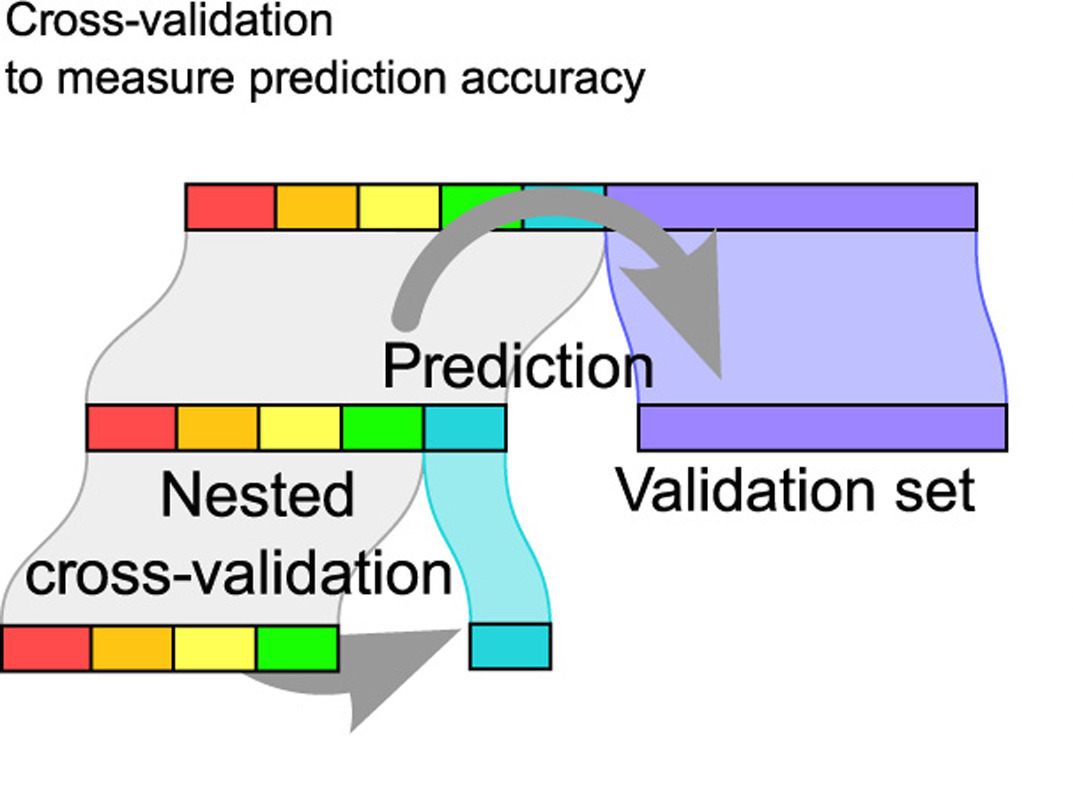
How does cross validation work?
Cross validation
More specifically, v-fold cross validation:
- Randomly partition the training data into v group
- Use v-1 groups to build the model (calculate MLEs); use 1 group for prediction / assessment
- Repeat v times, updating which group is used for assessment each time
Cross validation, step 1
Consider the example below where the training data are randomly split into 3 partitions:

Cross validation, steps 2 and 3
- Use 1 partition for assessment, and the remaining v-1 partitions for analysis
- Repeat v times, updating which partition is used for assessment each time

Cross validation using tidymodels
set.seed(4747)
folds <- vfold_cv(feeder_train, v = 3, strata = squirrels)
folds# 3-fold cross-validation using stratification
# A tibble: 3 × 2
splits id
<list> <chr>
1 <split [117841/58922]> Fold1
2 <split [117842/58921]> Fold2
3 <split [117843/58920]> Fold3Fit the model separately to each fold
feeder_rec1 <- recipe(squirrels ~ ., data = feeder_train) %>%
# delete the habitat variables
step_rm(contains("hab")) %>%
# delete the tree/shrub info
step_rm(contains("atleast")) %>%
step_impute_mean(all_numeric_predictors()) %>%
step_nzv(all_numeric_predictors())
feeder_rec1Recipe
Inputs:
role #variables
outcome 1
predictor 58
Operations:
Variables removed contains("hab")
Variables removed contains("atleast")
Mean imputation for all_numeric_predictors()
Sparse, unbalanced variable filter on all_numeric_predictors()feeder_log <- logistic_reg() %>%
set_engine("glm")
feeder_logLogistic Regression Model Specification (classification)
Computational engine: glm feeder_wflow1 <- workflow() %>%
add_recipe(feeder_rec1) %>%
add_model(feeder_log)
feeder_wflow1══ Workflow ════════════════════════════════════════════════════════════════════
Preprocessor: Recipe
Model: logistic_reg()
── Preprocessor ────────────────────────────────────────────────────────────────
4 Recipe Steps
• step_rm()
• step_rm()
• step_impute_mean()
• step_nzv()
── Model ───────────────────────────────────────────────────────────────────────
Logistic Regression Model Specification (classification)
Computational engine: glm metrics_interest <- metric_set(accuracy, roc_auc,
sensitivity, specificity)
feeder_fit_rs1 <- feeder_wflow1 %>%
fit_resamples(resamples = folds,
metrics = metrics_interest,
control = control_resamples(save_pred = TRUE,
event_level = "second"))feeder_fit_rs1 %>% augment() %>%
select(squirrels, .pred_class) %>%
yardstick::conf_mat(squirrels, .pred_class) %>%
autoplot(type = "heatmap") +
scale_fill_gradient(low="#D6EAF8", high="#2E86C1") 
collect_metrics(feeder_fit_rs1)# A tibble: 4 × 6
.metric .estimator mean n std_err .config
<chr> <chr> <dbl> <int> <dbl> <chr>
1 accuracy binary 0.809 3 0.000247 Preprocessor1_Model1
2 roc_auc binary 0.663 3 0.00180 Preprocessor1_Model1
3 sensitivity binary 0.996 3 0.000190 Preprocessor1_Model1
4 specificity binary 0.0265 3 0.000545 Preprocessor1_Model1Repeat the CV analysis for the second model
feeder_rec2 <- recipe(squirrels ~ ., data = feeder_train) %>%
  # delete the variables on when the birds were fed
  step_rm(contains("fed")) %>%
  # delete the variables about the bird feeders
  step_rm(contains("feed")) %>%
  step_impute_mean(all_numeric_predictors()) %>%
  step_nzv(all_numeric_predictors())
feeder_rec2Recipe
Inputs:
role #variables
outcome 1
predictor 58
Operations:
Variables removed contains("fed")
Variables removed contains("feed")
Mean imputation for all_numeric_predictors()
Sparse, unbalanced variable filter on all_numeric_predictors()feeder_log <- logistic_reg() %>%
set_engine("glm")
feeder_logLogistic Regression Model Specification (classification)
Computational engine: glm feeder_wflow2 <- workflow() %>%
add_recipe(feeder_rec2) %>%
add_model(feeder_log)
feeder_wflow2══ Workflow ════════════════════════════════════════════════════════════════════
Preprocessor: Recipe
Model: logistic_reg()
── Preprocessor ────────────────────────────────────────────────────────────────
4 Recipe Steps
• step_rm()
• step_rm()
• step_impute_mean()
• step_nzv()
── Model ───────────────────────────────────────────────────────────────────────
Logistic Regression Model Specification (classification)

Computational engine: glm metrics_interest <- metric_set(accuracy, roc_auc,
sensitivity, specificity)
feeder_fit_rs2 <- feeder_wflow2 %>%
fit_resamples(resamples = folds,
metrics = metrics_interest,
control = control_resamples(save_pred = TRUE,
event_level = "second"))feeder_fit_rs2 %>% augment() %>%
select(squirrels, .pred_class) %>%
yardstick::conf_mat(squirrels, .pred_class) %>%
autoplot(type = "heatmap") +
scale_fill_gradient(low="#D6EAF8", high="#2E86C1") 
collect_metrics(feeder_fit_rs2)# A tibble: 4 × 6
.metric .estimator mean n std_err .config
<chr> <chr> <dbl> <int> <dbl> <chr>
1 accuracy binary 0.813 3 0.000325 Preprocessor1_Model1
2 roc_auc binary 0.698 3 0.00228 Preprocessor1_Model1
3 sensitivity binary 0.990 3 0.000424 Preprocessor1_Model1
4 specificity binary 0.0693 3 0.000291 Preprocessor1_Model1Compare two models
Model 1
collect_metrics(feeder_fit_rs1)# A tibble: 4 × 6
.metric .estimator mean n std_err .config
<chr> <chr> <dbl> <int> <dbl> <chr>
1 accuracy binary 0.809 3 0.000247 Preprocessor1_Model1
2 roc_auc binary 0.663 3 0.00180 Preprocessor1_Model1
3 sensitivity binary 0.996 3 0.000190 Preprocessor1_Model1
4 specificity binary 0.0265 3 0.000545 Preprocessor1_Model1Model 2
collect_metrics(feeder_fit_rs2)# A tibble: 4 × 6
.metric .estimator mean n std_err .config
<chr> <chr> <dbl> <int> <dbl> <chr>
1 accuracy binary 0.813 3 0.000325 Preprocessor1_Model1
2 roc_auc binary 0.698 3 0.00228 Preprocessor1_Model1
3 sensitivity binary 0.990 3 0.000424 Preprocessor1_Model1
4 specificity binary 0.0693 3 0.000291 Preprocessor1_Model1Cross validation then test data
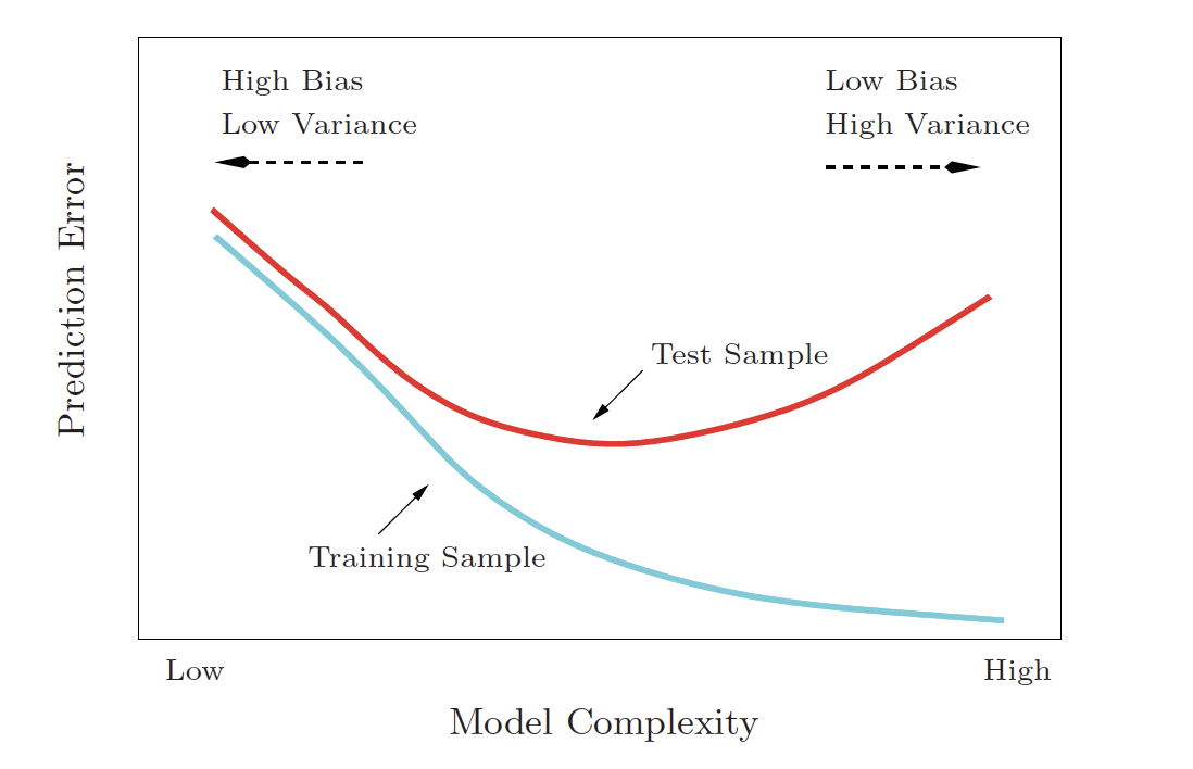
Bias-variance trade-off
References
Hastie, T., R. Tibshirani, and J. Friedman. 2001. The Elements of Statistical Learning. Springer.
Kuhn, Max, and Julia Silge. 2022. Tidy Modeling with r. https://www.tmwr.org/.
Varoquaux, G., P. Reddy Raamana, D. Engemann, A. Hoyos-Idrobo, Y. Schwartz, and B. Thirion. 2017. “Assessing and Tuning Brain Decoders: Cross-Validation, Caveats, and Guidelines.” NeuroImage 145: 166–79.